My name is Justin Beere, I am a student at UNISA. This is my submission for COS3712 - Computer Graphics Assignment 4.
This document is mostly the same as Assignment 2, I have added the new information to the lighting chapter, and added a texture chapter
I have always been interested in this subject and am happy to have had the opportunity to spend time learning to create 3d graphics on modern hardware.
Disclaimer: I am currently a software engineer, I know how to code and this is my original work. I did not copy code or ideas from any other student. The nature of the online material referenced may lead to similar code. While I tried to keep my code original and uniquely organised, WebGL has a specific API, and therefore code may seem similar to the implementations others have done. Please also note that some screenshots below might not look like the final result, I worked on this over many weeks and made many changes after taking the screenshots. Where code has been copied or adapted from other sources, I have noted it in the source file.
Unfortunately, it is not possible to load textures by opening the index.html file on your hard drive. You will see a lot of blue buildings like this.
In order for this to work, you will need to install node js and ‘live-server’ on your desktop.
sudo npm install -g live-serverlive-server in the directory where you unzipped the
project.In the meantime, to view the world without textures, you can toggle the buttons on the HTML page:
| key | action |
|---|---|
| Q | Increase Altitude |
| Z | Decrease Altitude |
| W | Move Forward |
| A | Strafe Left |
| S | Move Backward |
| D | Strafe Right |
| [ | Pause/Unpause Drones |
| ] | Pause/Unpause Cars |
Use your arrow keys to change camera direction.
Use any Mouse button to drag the viewport in different directions.
Use the scroll wheel to zoom in and out.
I decided to use HTML and JavaScript with the gl-matrix library for the highest likelihood of success, hopefully it will be as simple as opening the web page, no compiling required. I wanted to use Typescript as a language, for the benefit of a typing system, that also helps me to understand what I am doing, but decided against it, as it would involve a compiling step and I really wanted to keep this simple to run. Also, it was not an option in the assignment spec.
SceneGroup and and
SceneObject could have been more hierarchical, passing down
more complex matrix operations which would have allowed more complex
scenes and animations, it’s very simple in this version.pandoc -s -f markdown -t html5 -o doc.html doc.md -c doc.csspandoc -s --reference-doc=doc-template.docx --lua-filter=pagebreak.lua --from=latex+raw_tex -f markdown -o doc.docx doc.md
The index.html file describes the layout of the components on the screen. It initialises the Javascript code that in turn initialises the GL environment. It also houses the two shaders used to execute code on the GPU. From here I also import the gl-matrix library from an online cdn called CloudFlare.
I implemented the Javascript by using the ESM module system. This allows me to write plain Javascript and keep the code in different files that make sense. Unfortunately, this only works if you open the website over HTTP from an online URL, and not from your local file system. So as a compromise, I also bundle the code into a single Javascript file that is immediately invoked (iife). This way I can quickly develop the application, but then also bundle it so that the marker can open it from a file system like Windows Explorer. The index.html file takes care of this seamlessly (if it experiences an error loading the ESM module, it then executes the iife bundle instead), hopefully you don’t have problems running my web page!
Once the code is loaded and executed, the contents of
future-city.js are executed to initialize and run the WebGL
program.
The future-city.js function is called with the html
canvas element as a parameter. This canvas is then initialised to become
a WebGL view port.
const gl =
  canvas.getContext("webgl2") ?? canvas.getContext("experimental-webgl");
Hopefully this works for you when you open the page, I tested it in Chrome, Safari and Microsoft Edge on Mac and Windows 10.
Now I have the gl handle, I can use it to communicate
with the GL environment and the GPU.
As mentioned before, the code for the two shaders, the vertex shader
and the fragment shader, are in the index.html page. This is because the
browser makes it really difficult to load code from anywhere else. I
didn’t want to hard code the shaders inside Javascript, to me it’s
harder to read. So I wrote a helper function to load and compile the
shaders, it can be found int
src/utils/gl/create-shader.js.
The vertex shader is there to handle vertex coordinates, and the fragment shader is for determining the color of a fragment.
In WebGL, once you have 2 shaders, you can make a program. The
program is what GL uses to when rendering the current objects. I also
wrote a utility for this,
src/utils/gl/create-program.js.
In there I link the two shaders and verify that the program works.
Once I have the program loaded, I get the pointer locations for each of the input variables in the GL Program. These are declared in the shader code, and become the integration point between the CPU and the GPU, as this allows us to update variables in the program.
There are 2 types of locations in my project, attributes and uniforms. Attributes change their values based on the current vertex being read, and uniforms change their values based on the loop cycle being executed.
The next few lines of code instruct GL how to handle certain situations, such as depth testing (turn on), how to treat normals based on the order of the triangle vertices (counter clockwise). And what to do with faces that are not visible in the perspective (cull them).
Once all this setup is complete, I can start building the scene,for details, please read the sections on the Scene
After the scene is put into place, we can start rendering it. For
this I used the common method, which is to call
requestAnimationFrame with a callback, that then updates
variables based on time, renders the updated scene and then calls
requestAnimationFrame again.
requestAnimationFrame allows the browser to decide when the
next frame should be rendered, keeping the web page responsive while
also displaying these amazing moving graphics!
I broke the setup of all of this into seperate files for easier readability and maintainability.
future-city-buildings.jsfuture-city-drones.jsfuture-city-landscape.jsfuture-city-roads.jsfuture-city-space.jsfuture-city-vehicles.jsEach of these files create an array of SceneGroups, each
SceneGroup is then a collection of related
SceneObjects.
I go into more detail of how models are loaded and sent to the GPU under Modeling.
The requirements for the project were to create a city scape, with a ground plane, buildings and vehicles.
The landscape is made up of a plane (that I generated myself), this plane has a function on the y-axis that allows for the effect of different heights at different positions on the xz-plane. The color of the plane is also a function of the y-axis, which create beaches and rolling grasslands. I then created a second plane that represents water, and allowed it to clip into the “land” plane below the xz-plane. This gave the effect of a river running through the landscape. I even animated the water (sine wave on the y-axis) to give the effect of tides on the beaches.
(These were all done while I was learning to generate this plane, and the power that mathematics has in this world!)
I found a model of a simple tree and imported into my project. I then used this model to add some more green to the landscape. It is rotated on the y-axis for variety, and laid out by translation as if done by a city planner.
I created a large black plane and then covered it in smaller grey planes to give the effect of roads and concrete city blocks. This would form the layout of my city, where the buildings and vehicles would go…
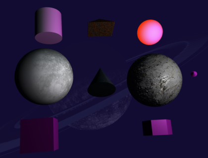
Once I had all my primitives working and able to be transformed and animated, I could go to work creating various buildings for the scene. The project spec wanted me to demonstrate using the various matrix transformations to create a variety of buildings. I used spheres, cylinders, cones, cubes, octagons and pyramids to create these. I introduced dynamic effects by using rotations, translations and scaling, some of the building components are even animated. I hope I used enough technique for these buildings.
There are 8 buildings in the scene. Some are reused, with some transformations applied, and others vary from complex to pretty simple. I had to do this while keeping the city looking organised and purposeful, and keeping in mind that the second part of this assignment is to add lighting and textures.
There is space for more buildings, but this creative part is very time consuming and I now realise why it takes so long to develop games with complex and interesting scenery.
I was also asked to create at least 4 flying cars and make them move along paths. I designed the cars in Blender (I am not great at 3D modelling!). They don’t have wheels so I guess they can fly. If you zoom in on them, you will see they are slightly translated up the y-axis, so they float at least. I have a few cars, more than 4, and they all follow distinct paths through the city. I explain how they follow their paths under Animation. They also travel at different speeds along the roads of the city.
There is a pause function for them. If you click “Pause Cars” they will stop animating and just sit there, waiting for you to click the button again to unpause them. I explain this process under Animation too.
I needed to have 4 hovering drones that “rotate in place”. I made up a model using toroids and triangles for propellers. The propellers are spinning and this is my interpretation of rotating in place. They also have a bit of a floating animation applied to the whole drone.
There is also a pause button for two of them, if you click “Pause Drones” you will see that they stop floating and their propeller blades stop rotating. If you click the button again, they will continue.
The project requires us to use geometric primitives to build up more complex objects. So, I had to come up with a way to get meshes of vertices onto the GPU, and into my 3D world!
OpenGL/WebGL provide APIs to load buffers of data into the RAM on the GPU. In the simplest form this is done with the following steps:
const vertexBuffer = gl.createBuffer();
// a simple buffer that is an array of elements on the GPU
gl.bindBuffer(gl.ARRAY_BUFFER, vertexBuffer);
// send the vertex model to the GPU
gl.bufferData(gl.ARRAY_BUFFER, vertices, gl.STATIC_DRAW);
This copies a buffer of data from memory on the CPU onto the GPU for rendering. This buffer needs to be structured in such a way that each vertex and all extra information associated with it are together.
The format that I used for all models in this project is as follows:
[
  ...,
  vx, vy, vz, nx, ny, nz, cr, cg, cb, gr, gg, gb, s, nnx, nny, nnz // vertex n
  vx, vy, vz, nx, ny, nz, cr, cg, cb, gr, gg, gb, s, nnx, nny, nnz // vertex n+1
  vx, vy, vz, nx, ny, nz, cr, cg, cb, gr, gg, gb, s, nnx, nny, nnz // vertex n+2
  ...
]
Where:
vx, vy and vz are the 3d
coordinates of the vertex in relation to the origin of the modelnx, ny and nz are the 3d
components of the vector that points 90 degrees away from the face of
the vertex (for flat shading)cr, cg and cb are the red,
green and blue components of the color of the vertex (and face)gr, gg and gb are the red,
green and blue components of the glow of the vertex
(and face)s is the value for the shininess of the facennx, nny and nnz are the 3d
components of the vector that points in the natural direction that light
should reflect from the vertex (for gouraud shading)It is worth noting here that three of these vertices make up a triangle, which make up a face of the model, and usually they all have the same normal and color values. In the second part of this assignment I want to play around with having different colors on the same face, and also even different normals on the same face for different effects. Also a future layout may include more data, such as texture maps, bump maps, and a “glow” effect that I thought of but decided not to implement at this time.
You also need to let GL know how to intepret this buffer, and there are APIs for that too:
gl.enableVertexAttribArray(positionAttribLocation);
gl.vertexAttribPointer(
  positionAttribLocation, // pointer to the position attribute in the shader
  3, // number of elements for this attribute
  gl.FLOAT, // type of element
  gl.FALSE,
  9 * Float32Array.BYTES_PER_ELEMENT, // total size of a vertex
  0, // offset (the position is first)
);
The above code tells the GL how to extract information in the buffer.
In this case I am telling it that a vertex array is 9 elements long, and
that the position coordinates for the vertex are in the first three
entries in the the array. And the for each vector, this will be loaded
into the positionAttribLocation pointer in the shader. Note
that the correct buffer must be bound so that GL knows
which buffer you are talking about.
The same must be done for the normal attribute:
gl.enableVertexAttribArray(normalAttribLocation);
gl.vertexAttribPointer(
  normalAttribLocation, // pointer to the normal attribute in the shader
  3, // number of elements for this attribute
  gl.FLOAT, // type of element
  gl.FALSE, // not sure what this is
  9 * Float32Array.BYTES_PER_ELEMENT, // total size
  3 * Float32Array.BYTES_PER_ELEMENT, // offset (normal is from element #3)
);
Where now, the normal is offset 3 elements and is also 3 elements long.
And, of course, the color attribute:
gl.enableVertexAttribArray(colorAttribLocation);
gl.vertexAttribPointer(
  colorAttribLocation, // color attribute location
  3, // Number of elements per attribute
  gl.FLOAT, // Type of elements
  gl.FALSE,
  9 * Float32Array.BYTES_PER_ELEMENT, // total size of vertex
  6 * Float32Array.BYTES_PER_ELEMENT, // offset (color is from element #6)
);
In case you are wondering how this relates to code the vertex shader:
// X Y Z start position of the vertex, from the local model's origin
in vec3 aPosition; // positionAttribLocation
// X Y Z normal of the vertex
in vec3 aNormal; // normalAttribLocation
// R G B color of this vertex
in vec3 aColor; // colorAttribLocation
// color of glow
in vec3 aGlow;
// shininess of surface
in float aShininess;This data buffer needs to come into existance somehow, so I came up with a simple functional interface that allows me to use a model exported from blender, or generate the model on the fly.
export default (colour, /*other parameters*/)) => {
  // once off setup
  return () => { // second (lazy) function
    // generate an array of data in the following format:
    const vertices = [
      ...,       // previous vertex
      vx,vy,vz,  // vertex in 3d space, relative to a local origin
      nx,ny,nz,  // normal, the orthogonal, normalized vector from the face that this vertex belongs to
      cr,cg,cb,     // color, red green and blue values for the color of the face
      gr,gg,gb,     // color, red green and blue values for the glow of the face
      s,            // shininess
      nnx,nny,nnz,  // normal, the average, normalized vector from vertex
      ...        // next vertex
    ];
  }
}
The first function is for once off configuration of the model, where parameters such as color are passed in
The second part, when called lazily, generates an array of 16 values per vertex:
Each model will have a different algorithm to generate the vertex
buffer. Or they may be exported from Blender in a hard coded array. You
can find these models in the project under
src/models/*.js
While I was learning about this process of rendering objects in Computer Graphics, I realised that there are some things that the CPU does better than the GPU. The GPU can be thought of as an array of very small specialised CPUs. They do some things really well, and very fast, and in parallel. But they should be used sparingly for what they are good at. Other, less frequent transformations are still better off done on the CPU.
For example, generating a model, and then doing a once off transformation (applying a transformation matrix to all the vectors in a model) can be done on the CPU. These transformations include operations such as scaling, translating and rotating. This process involves the following steps:
This process is different from doing it on the GPU, because the already transformed model is sent to the GPU for rendering. If this were left to the GPU, it would need to perform these operations on each and every vertex in the scene for every frame rendered, which would be a waste of time as nothing would change.
For these CPU calculations, I used the gl-matrix
library, which is a well known javascript implementation for many useful
Linear Algebra functions. I did ask Dr Lazarus in an email if I may do
this and he agreed.
gl-matrix may internally implement things differently to
what we see in a course such as MAT1503, but these would just be
optimisations on the same concepts.
Here is a screenshot of my first cubes that had some transformations applied to them as individual models:
In order to get from an individual vertex to a scene of moving objects and perspectives, what seems to be a lot of things need to take place. These operations are executed one after the other in a pipeline, each step having a different function on the 3d world.
Most of this work is to try to find out where every vertex in a world of 3d models should appear on the 2d view that your display provides.
// calculate vector position
gl_Position = uProj * uView * uModel * vec4(aPosition, 1.0);
This is accomplished by simply taking a set of matrices, that each represent some aspect of what we want to render, and performing matrix multiplication on them in reverse order from:
aPosition: the position of the individual vertex in 3d
before the transformationuModel: the position and orientation of the model that
the vertex belongs to, any transformations in this matrix will apply to
all the vertices in the model at once, this includes animation of the
modeluView: the position of the camera in the world. this
matrix will have the effect of viewing the world from different angles
and locationsuProj: the final projection onto a 2d view port// X Y Z start position of the vertex, from the local model's origin
in vec3 aPosition;
// the matrix that will transform the object locally
uniform mat4 uModel;
// the matrix that will put this vertex into a position on in the view
uniform mat4 uView;
// the matrix that will put this vertex into a position on the raster
uniform mat4 uProj;The aPosition variable is prefixed with an
a because it is an attribute obtained from the model array
of vertex information. It generally does not change during the lifetime
of the application.
The other matrixes, prefixed with a u are uniform
variables, this is to ideintify them as variables that can be updated
between frames, but are the same for all vertices.
In the section for Modeling I describe how to
get the individual vertices into the aPosition field in the
shader. In my project, this is done once per vertex, and is never
updated again. To move the vertex around, we use the other matrices.
In the section for Animation I explain how
we modify and update the uModel matrix in the render loop,
to move and rotate the model in a variety of ways, to effectively move
and orient an entire model in the scene.
In the section for Camera I explain how
modifying the uView matrix has the effect of moving the
user perspective, or camera around inside the world. It has the effect
of moving all models around in the field of view.
In the section for GL Setup I explain the
uProj matrix. It does not change after the initial display
of the world.
I implemented an animation framework from scratch. The concept is fairly simple, we can ask a question: what must the transformation matrix look like at a specific time?
The basic interface for an animation is an array of sub-animations, that will pass a transformation matrix along the animation pipeline, modifying it as it goes. The final output is a matrix that can be applied to all the vertices of the model. The factor the causes this matrix to change over time is time itself. So the matrix produced at one moment may be different to one produced at another moment.
The animation loop provides us with some opportunities to modify the scene at some interval. If everything is going well, and the application is performant, this interval is only limited by the refresh rate of the monitor you are viewing it on.
Early on in development, I used a technique to display the current “FPS” or frames per second on the application user interface. The way that this is done, is by calculating the amount of time that has passed since the previous frame was rendered and converting that into FPS. This number is useful for development, as I can monitor it to ensure that the only bottleneck is the refresh rate of the screen. My screen at home has a 60Hz refresh rate, and if the FPS goes below that, I know I have done something to degrade the performance of the app. Hopefully you see your screen’s refresh rate in the FPS field!
let last = performance.now();

var loop = function () {
  // calculate the frames per second for display
  const time = performance.now();
  const elapsed = (time - last) / 1000;
  last = time;
  const fps = 1 / elapsed;
  fields.fps.innerText = fps.toFixed(1);
  // ... other rendering code
};performance.now() gets the number of milliseconds since
the web page was opened. This provides a deterministic value that is the
same every time you refresh the page. An alternative would be
new Date().getTime(), but that is the number of
milliseconds from a fixed point in the past. I chose
performance.now() because I wanted to be able to see
certain animations happen in a predictable way during development. If
two cars bump into each other after 10 seconds, I want that to happen
again if I refresh. The other way, I would never see the same animation
again unless I reset my PC clock!
This moment in time changes for each animation frame, and is not dependent on the frame rate. So when I use it for animation, vehicles and drones will travel across the screen at the same rate, no matter how powerful your graphics card is, or how fast your monitor can refresh.
I implemeted this by providing an animation pipeline interface, which
accepts an array of distinct animation functions that will build upon
each other. For example, I can pass two animations to the the pipeline,
fly-circle, and wave. fly-circle
will move the object around an origin point, while keeping the model
facing in a logical forward direction, and then the wave
animation will translate the model up and down in a smooth sine wave.
Together these animations provide the effect of flying in a circle, and
bobbing up and down at once.
// the wave animation function
export default (height, speed) => (init, model, time) => {
  // calculate the current height of the object
  const locationY = Math.sin((time / 100000) * speed) * Math.PI * height;
  // move the object to that location (by updating the translation matrix of course)
  mat4.translate(model, init, [0, locationY, 0]);
  // no normals were hurt during this transformation
  return false;
};
This is achieved by passing a 4x4 identity matrix though the pipeline, giving each animation function an opportunity to apply transformation operations to it. After the pipeline, the matrix has a transform for that moment in time, that can be applied to each vertex (and normal) in the model. If this is done many times a second, the effect of animation has been achieved.
You can find all the different animation functions under the
src/utils/animate directory.
In the assignment spec, there is the requirement to pause/unpause
certain animations when a button is pressed. I implemented this by
adding a shared “pause” object. Which is simply an array with a single
boolean. When this boolean is true, the animation stops. The
animate pipeline simply skips the animation loop. When it’s
false the animation pipeline continues. During animation,
how much “unpaused” time is passed is recorded. This way, when we are
animating, we are no longer using the raw input time, but the time
accumulated when unpaused. This has the effect of continuing where
you left off after pausing.
// animation pipeline
export default (steps, pause = [false]) => {
  // accumaulate the actual time that this animation has been unpaused
  let unpausedTime = 0;
  // the last real time
  let lastTime = 0;
  return (init, model, time) => {
    if (!pause[0]) {
      // if not paused
      unpausedTime += time - lastTime;
      // reset the matrix
      mat4.copy(model, init);
      // run the matrix through the pipeline for this moment in time
      steps.reduce(
        (normalsAffected, step) =>
          // do each step, and record if normals were ever affected
          step(model, model, unpausedTime) || normalsAffected,
        // were the normals updated?
        false,
      );
    }
    // remember the time for next time
    lastTime = time;
  };
};I implemented this by creating an animation step function that does a few things.
It can go in a straight line, it can turn left, and right.
Going in a straight line is simply translating in a certain direction over time. So at a given point in time, the object will have translated over a certain percentage of distance.
Turning left and right does the same thing, but along a curve from 0
to 90 degrees. The curve distance is therefore
(Math.PI / 2) * radius. We can calculated how far along the
curve the object is by using this formula with the elapsed time.
The overall segmented path controller has an array of these segments, and can index the path that the object is in, based on the current time. Once the current segment is determined, that segment is asked to modify the transformation matrix, which involves translation and rotation. The overall effect is a smooth path of lines and turns.
I also created a “builder” for these paths, to make it easy to code the path for a certain vehicle.
All this code can be found in
src/utils/animate/segmented-path.js
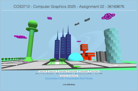
To be able to explore the city, I needed to be implement ways to input movement controls into the world. I implemented this using HTML buttons and keyboard and mouse input.
The camera has 3 vectors associated with it, position,
direction and lookAt.
position is the coordinates of the camera in relation to
the world origin. direction is a unit vector in the
direction that the camera is facing. lookAt is the
coordinates of the position that the camera is looking at, it is the sum
of the position and the direction vectors, i.e the point directly in
front of the camera.
These three variables are modified by different inputs, and
ultimately modify one of the main graphics pipeline matrices, the
viewMatrix. I covered the role of the View Matrix under
Vertex Shader.
The effect of changing the translation and rotation of the
viewMatrix is that the viewer perspective is able to move
and look around inside the world, this really makes the 3D world into
something that can be explored!
To change the position of the camera, we need to move in a specific direction. For each direction we need to calculate a vector based on the camera direction and add the resulting vector to the position vector. If we do this repeatedly, this creates the effect of movement.
-1Math.PI / 2 (90 degrees) from the
camera direction vector(Math.PI * 3) / 2 (270 degrees) from
the camera direction vector(0,1,0)(0,-1,0)To simulate looking around, I repeatedly rotate the camera direction vector by some small angle (theta), on the appropriate axis:
I did look into using quaternions for this, but decided against it, maybe the second half will use them, as I honestly just don’t understand it for now
In HTML user input is captured by listening for various events from the user. These events contain enough information to figure out what to do. After calculating a new direction and/or location for the camera, my code fires another event to notify the camera controller to update the viewMatrix, which will be sent to the shader and processed in the Grpahics Pipeline on the next render loop.
Coming up with good camera input controls was tough, I tried my best to do something intuitive.
(The following may have changed since I wrote this I hope I remember to update it before submitting!)
I added 6 buttons to the html page:
Each of these buttons represents a hard coded direction,
and location, and when clicked, will modify the camera and
notifiy the controller to update the viewMatrix for the
next render.
To find the code for these buttons:
src/camera/camera-buttons.js
Try them out, I hope you like the city views that I selected.
Having static locations is one thing, being able to control the camera yourself is another.
To find the code for these buttons:
src/camera/camera-keyboard.js
Adding mouse controls just take the robotic keyboard motions and make them fluid. The user can now finely control the direction of the camera!
While holding down any mouse button over the world canvas, move your mouse. Hopefully the resulting movement is intuitive enough.
I implemented this by keeping track of how much the mouse has moved between each event. The delta between the mouse positions are used to calculate an angle on the x-axis and another angle on the y-axis. These two angles are then used to calculate a new direction for the camera.
I did use quaternions for this, which allows for smooth movement on 3-axis with only 2 angles, as the mouse only moves in 2D
Use the scroll wheel of your mouse to move forwards and backwards in the world. This uses the same technique as the forward and backward buttons on the keyboard, except the delta between scroll events is used to scale the movement vector.
To find the code for the mouse:
src/camera/camera-mouse.js
Not implemented, I would like to implement this in the future, so that you can navigate the world on your phone too!
In order for the world to be at least vaguely interesting, I would need to implement at least some lighting. Even though it was not required for the 1st part of the project.
I added a few fields to my vertex shader:
// The direction of the sun
uniform vec3 uSunDirection;
// The color of the sun
uniform vec3 uSunColor;
// Color of the ambient light
uniform vec3 uAmbientColor;
For the first part of the project, these will be initialised once. Later on we need to be able to update these to simulate different times of day.
For now though I implemented basic sunlight angle and color and general ambient color.
To get this to work, each vertex in the model needs to have a normal for each face it belongs to. For this reason, and to keep it simple, I had to abandon the technique of using indexed vertices. An indexed vertex can only have one set of extra data associated with it. My data format for this stage of the project is [[vertex],[normal],[color]], and so one vertex, one normal, one color. But if the vertices are shared between faces, it’s not possible to have more than one normal, and so I need to duplicate the vertices. This makes the model arrays a bit bigger, but for this project, that is ok.
// X Y Z normal of the vertex
in vec3 aNormal;
// R G B color of this vertex
in vec3 aColor;
For animated objects, the current transformation that has been applied to vertex must also be applied to the normal. This is achieved by calculating the inverse transpose of the transformation matrix, and applying it to the normal. This calculation, along with the calculation of the transformation matrix, is done on the CPU and not in the shader, as it only needs to be calculated once for the entire model. If it was implemented on the shader, this would not be efficient, as the same matrix would result for every vertex in any case.
I then pass this matrix to the shader as uNormal:
// precalculated normal matrix for this model (and vertex)
uniform mat3 uNormal;
The normal is the vector perpendicular to the face of the plane that we are rendering. So each vertex on the face (in our case there are always 3) has the same normal. This way all the vertices on the triangle will have the same final color. We can use this angle to calculate how strongly a directional light will light up the surface, with some linear algebra:
// calculate face color
vec3 normal = normalize(uNormal * aNormal);
float diffuseStrength = max(dot(normal, uSunDirection), 0.0);
vec3 diffuse = uSunColor * diffuseStrength * aColor;
vec3 ambient = uAmbientColor * aColor;
vColor = ambient + diffuse;
First we calculate the current transformation on the normal by multiplying it with the current transform. Then we can calculate the strength of the directional light using the dot product of the normal and the direction of the sun. This gives us a scalar “strength” from 0 to 1. Where 1 would be maximum brightness (90 degrees), and 0 would not light up the surface at all. We then take that strength and multiply combine the color of the light and the color of the surface. The last step is to brighten up the entire object by adding the ambient color to it.
For models exported from Blender, I had to go through a process to convert the model into the format I chose for this project.
Below is new documentation to do with the objectives for Assignment 4.
In part one of the project, I implemented a basic directional light that simulated sunlight. In part two I implemented an animated directional light, that makes use of the system time to calculate the direction of the light at any moment, this is updated during the animation loop and gives the effect of sunrise, afternoon, evening and night time. There are also buttons to switch between the times of day, instead of waiting for the animation to get there.
There are 5 buttons:
Clicking any of the first 4 will change the daylight to simulate the lighting for that time of day and pause it. The Auto button then resumes the animation when clicked.
The different times of day also have ambient mappings to change the tone and mood appropriately. At night, the ambient color goes very dark, to allow the other lighting effects to take over.


Here is the implementation of the addDirectionalLight
GLSL function.
vec3 directionalLight(
vec3 N,
vec3 V,
DirectionalLight light,
float shininess,
bool hasSpecular,
vec3 albedo
) {
vec3 L = normalize(-light.direction);
LightingCalc lr = calcLighting(N, L, V, light.color, shininess, 1.0, albedo, hasSpecular);
return lr.diffuse + lr.specular;
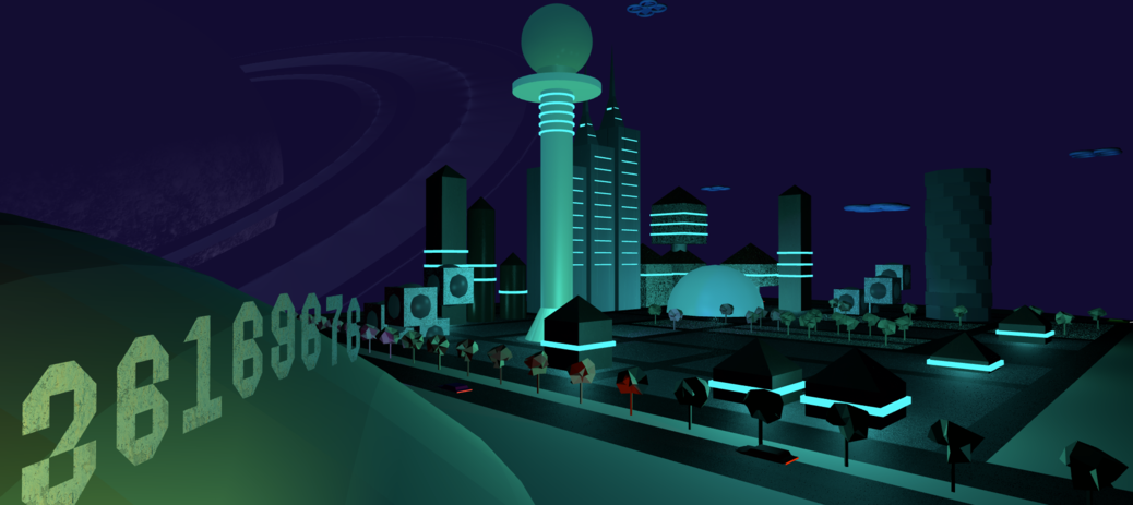
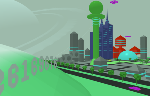
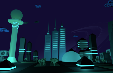
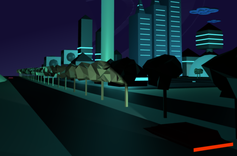
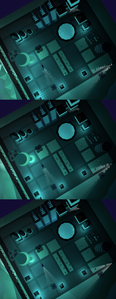
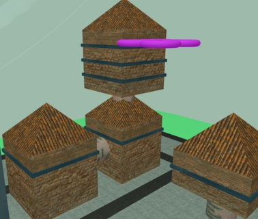
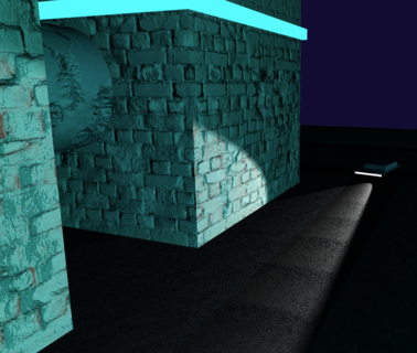
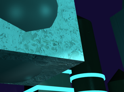
}I decided to use point lights to light up the city at night, I placed them inside specific buildings, to create the effect that the building was glowing. Since this is a futuristic city, why not let the buildings themselves be street lights? So inside the tower, and inside the sphere building in the center of the city, there are point lights. The buildings themselves have a glow effect applied, to really make it seem like they are lighting up the city, and not point lights. I will discuss the glow effect a bit later.
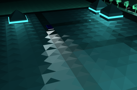
In the screenshot below, you can see the buildings on either side, on the left, a tall “sucker stick” and on the right, a great sphere, that are glowing and lighting up the buildings around them. There are also several smaller building that have point lights inside them, lighting up their area.
Here is the implementation of the addPointLight GLSL
function. It calls the calcLighting function (in a future
section).
vec3 addPointLight(
      vec3 N,
      vec3 V,
      vec3 P,
      PointLight light,
      float shininess,
      vec3 albedo
  ) {
  // calculate the distance from the object position
  vec3 L = normalize(light.position - P);
  float d  = length(light.position - P);
  float att = 1.0 / (1.0 + 0.09 * d + 0.032 * d * d);

  // use this to calculate the lighting (including binn-phong)
  LightingCalc lr = calcLighting(N, L, V, light.color, shininess, att, albedo, true);
  return lr.diffuse + lr.specular;
}
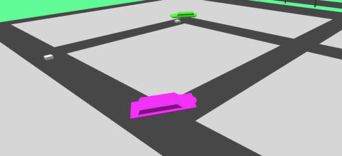
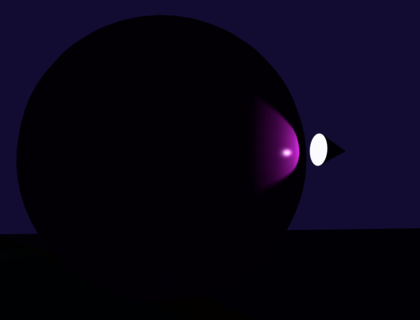
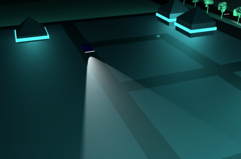
I added spot lights to the moving vehicles. In my scene, I have 8 cars that drive around the city. Each of these has a spotlight in front and pointed in the same direction as the vehicle. I implemented this by applying the same animation to the point light as to the vehicle. This gives the effect of the vehicle having a light attached to it. We can see how the lights light up parts of the city and landscape as they translate and rotate along their paths.
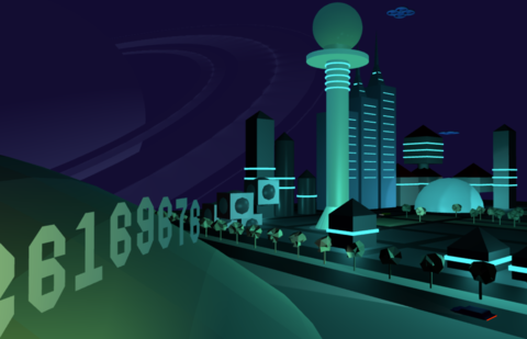
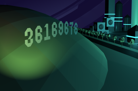
I also added some more spotlights that light up my student number on a dark hill.
Here is the implementation of the addSpotlight GLSL
function. It calls the calcLighting function (in the next
section).
vec3 addSpotLight(
      vec3 N,
      vec3 V,
      vec3 P,
      SpotLight light,
      float shininess,
      vec3 albedo
  ) {
    // calculate the distance from the object position
    vec3 L = normalize(light.position - P);
    float d  = length(light.position - P);
    float att = 1.0 / (1.0 + 0.09 * d + 0.032 * d * d);

    // calculate the size of the cone shape
    float cosTheta = dot(L, normalize(-light.direction));
    float epsilon  = max(light.cutoff - light.outerCutoff, 0.0001);
    float cone = clamp((cosTheta - light.outerCutoff) / epsilon, 0.0, 1.0);

    // use this to calculate the lighting (including binn-phong)
    LightingCalc lr = calcLighting(N, L, V, light.color, shininess, att * cone, albedo, true);
    return lr.diffuse + lr.specular;
}
There was a requirement to showcase different shading methods, and also the ability to switch between them while the application is runnning. There were a couple of strategies I could have used, including adding extra uniforms to select different code in a single shading program. I think this would have worked, but having a lot of logic in my shaders was too risky, especially since shaders are very difficult to debug. So I went with the approach of creating a distinct program for each shader technique.
There are 3 buttons:
Clicking these buttons will change the program on the fly, effectively using the new program to render the next animation frame, and you will be able to see the differences visually. It is also useful to use the pause buttons to stop an interesting object from moving while swithing shaders.
There were a few things that I had to do to get this to work properly:
gl.useProgram(programX)Importantly, the shaders are compiled once when the program starts up, and then they are kept in memory to be switched quickly.
Originally, the application used flat shading to render the scene. The big difference between all the shading types is how the normals relate to the faces and vertices of the 3d models.
I used a common algorithm to implement flat, gouraud and phong
shading, even though they are calculated at different times, and use
different types of normals. Here is the implementation for the
calcLighting that is used by all three lighting types:
LightingCalc calcLighting(
vec3 N, // the normal vector (after interpolation for fragments)
vec3 L, // the direction of the light
vec3 V, // the direction of the camera
vec3 color, // the color of the light
float shininess, // the shininess of the material
float attenuation, // the intensity of the light
vec3 albedo, // the original color of the material, before any lighting is applied
bool hasSpecular // completely disable blinn-phong for certain materials
) {
// result has two outputs, diffuse and specular
LightingCalc result;
result.diffuse = vec3(0.0);
result.specular = vec3(0.0);
// intensity of diffuse light
float ndotl = dot(N, L);
// saturate diffuse intensity
float diffuseIntensity = clamp(ndotl, 0.0, 1.0);
// add up the total light generated for diffuse light
result.diffuse = albedo * color * diffuseIntensity * attenuation;
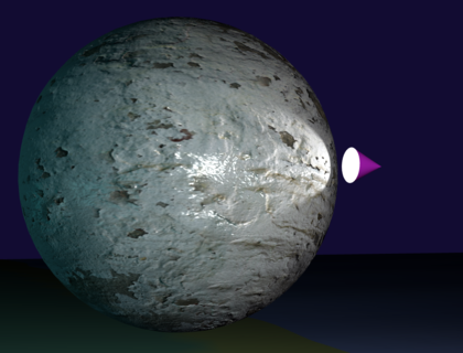
// for some models we don't want specular (like for moons outside of the atmosphere)
if (hasSpecular) {
// blinn-phong
// calculate the half vector between the light vector and the view vector.
vec3 H = normalize(L + V);
// intensity of the specular light
float ndoth = max(dot(N, H), 0.0);
float specularIntensity = pow(clamp(ndoth, 0.0, 1.0), shininess);
// add up the total light generated for specular light
result.specular = color * specularIntensity * attenuation;
}
return result;
}For flat shading, the normals of vertices are split. In other words, vertices do not share a normal. The normal is the same for each vertex on a given polygon. Because of this, from a lighting perspective, each vertex belongs to a face, and that face is lit up in the same way across itself. So the effect is the entire polygon having the same final color.
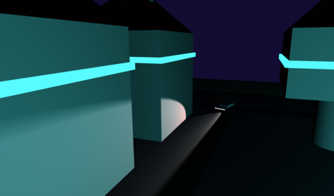
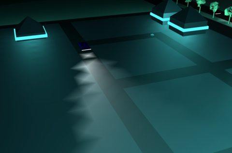
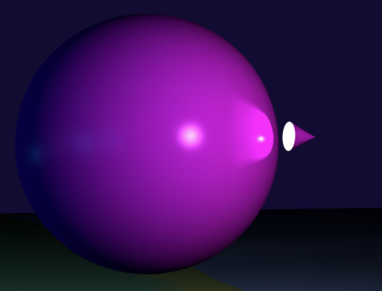
Technically, all the processing for the flat shader is done in the vertex shader, and not in the fragment shader. This results in inaccurate lighting, but is also a lot faster, as there are less vertices than fragments to process. The fragment shader has been set to not interpolate the colors, which can result in some strange effects. Like in the next image you can see how the car’s head lamp lights up the road in a peculiar way:
Gouraud shading improves on flat shading by doing the same processing, but with a different type of normal. Now instead of all the normals of a face pointing in the same direction, now, all the normals that share a vertex point in the same average direction. The effect of this is that the final color is not the same across the face, resulting in a smoother interpolation of the color.
Phong Shading, like Gouraud shading, also uses normals that are shared between vertices, but does the color processing in the fragment shader, this results in much higher fidelity reflections and colors. But because a calculation needs to be done for every fragment, it’s much more processor intensive. The results are much prettier though, compared to flat and gouraud shading. You can see here how smoothly the car headlight lights up the roads now.
Flat shading (top) produces edgy looking models, if you are into that sort of thing. The specular highlight is not visible. The blocky look is gone in the Gouraud shader (middle), and the specular highlight is more visible. Notice the crisp the specular highlights are on the Phong shader (bottom), almost realistic.
If you are viewing this in the Word doc, then the entire image may not be visible, I could not get a high enough quality comparison to fit onto a page! Please use a different view mode, or open the HTML documentation.
I wanted the night city to have a style and look like one of my
favorite movies: Tron 2. That movie incudes a lot of glowing blue
lighting and I think it looks amazing. To create a similar affect I
added a new attribute to my vertex data, that is an RGB value. There is
also now a new uniform called glowBrightness that is send
to the shader before every frame is rendered. This brightness is
calculated based on the time of day, at night it is bright and during
the day it is not. As the scene darkens, these glow effects take over
from sunlight. Combined with point lights, this produced a very
satisfying effect, I think.
The glow was also useful for making other lights pop at night, such as the exhaust and spotlights of the flying drones, and the headlights and taillights of cars.
This part of the project took by far the longest. It took my some time to undertand how UV mappings work. And then I had to update my model vertex layout to include the UV coordinates for each vertex, and also the precalculated tangent vector for each face. Once I had textures and bump maps incorporated into my world, I had to try to stop myself from just adding more and more!
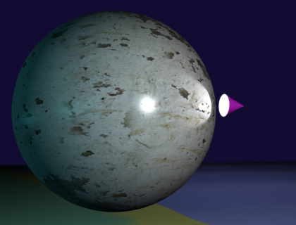
I found a great resource for textures at polyhaven.com. Here I could find some free textures that also included the correct normal mappings for them.
In order to get textures to work, I had to do a few things. I had to update my vertex buffer layout to include a new field, a 2D vector for UV mapping. This could then be used in the fragment shader to map the cooridnates to a texture file, to produce a color for that fragment. So I found some texture files online, and added them to my project. I wrote some code to load the textures onto the GPU. Each texture has it’s own file, and multiple models can share a texture.
Example of a texture:

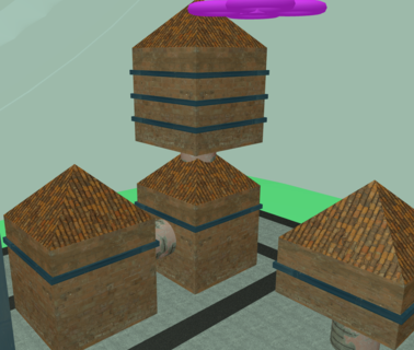
We went from no textures:
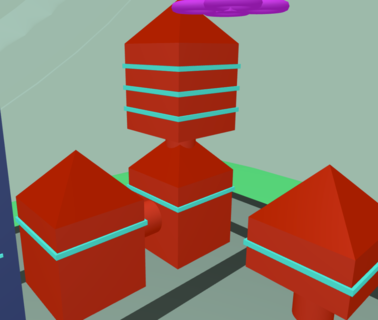
To having textures:
In order to apply bump mappings, I also had to add a 3D vector for the surface tangent to my vector layout. This new field, together with the UVs and the normals (I already had from gouraud shading), we could create a new matrix called a TBN. TBN stands for tangent, bitangent and normal. These 3 vectors can be used to produce a 3D matrix, that allows us to transform the vectors in world space over a bump map. This produces new vectors acorss the face of the object, that gives the illusion of very detailed meshes.
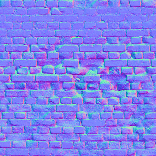
The bump map contains 3D vectors, encoded as RGB values in a PNG image. We can read these in as a texture map, but instead of usng the colors you see above, we can transform the surface normal of the fragment, to produce a stunningly detailed effect.
Here are some closer shots of the bump effect:
If you do not see textures in the live demo, please check to see that the buttons “Diffuse Textures” and “Bump Maps” are on.
Also, see the note at the beginning of this document, textures cannot be viewed when a web page is loaded from the file system. You will need to install a server and run it from there. Apologies, this is a security limitation that browsers have implemented.
In a hidden part of the scene, I included some test objects that I used while developing, to see what happens.
You can access it by clicking the “Camera TEST” button.
There you can use the other buttons to see the effects of different configurations, animations, ligthing, textures and models.
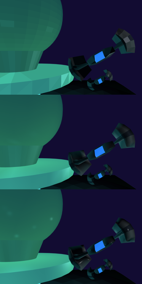
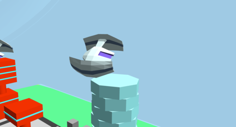
When I read the spec for this assignment, I immediately thought of a scene from “Second Reality”, a demo showcased at the “Assembly ’93” computer graphics show. This demo was implemented by a team of young developers called “Future Crew”. Since being a teenager, I have been super inspired by this demo, and I decided to model one of the drones after a 3D craft that featured in the closing scene of the demo over 32 years ago.
YouTube: Future Crew - Second Reality (1993)
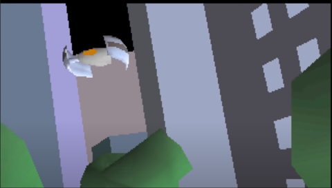
I used blender to import the original model that can be found here: Second Reality Github Repo
The model is in an old 3DS Max format, and not 100% compatible with Blender. I had to go through a fair number of steps to get the model into a format suitable for importing into my project, but eventually I managed to bring the old drone back to life!
the model I used here and all the source code in the Second Reality Github Repo is public domain and free to use by anybody for any reason
I spent well over 100 hours on this task. I really enjoyed learning about WebGL and how to apply Linear Algebra to modify this world in many different ways.
I am looking forward to giving my world some serious upgrades,
with more complex lighting, textures and bump maps.
Done!
If you feel that I may have plagiarised any part of this project with another student, please let me know. I have proof of work on my Github account, which is in a private repository currently, as I do not want others to have access to my work before the due date. I have not interacted with any other students of this module, I don’t even know if there are any others.